Some R basics for SPSS users
There are a lot of reasons to use R instead of my field’s standby software, SPSS. With that said, I won’t get into them here. Instead, I just want to talk about a few things in R that might help a beginner get the hang of it.
If you’re moving from SPSS and are just a social scientist with no particular training in things like programming, here’s what you should know about R:
- There’s no point-and-click interface; virtually everything you need to do will be done via written code.
- Don’t expect to sit down one day with no experience in R and be running production-quality analyses within a few minutes. Quick learners and those with some programming experience will pick it up fairly quickly, but give yourself some time to learn how things work. You will inevitably get stuck on a seemingly simple problem and take way too much time trying to sort it out.
- R will likely change the way you think about data analysis. When you have to write code to make things happen and that code is in R, you’re likely to think about the data and what you can do with it in a different way than you do if you have only used SPSS. This is good!
Before we get started here, I should mention that I will not write about how to install R. I have nothing to add beyond the many resources on this topic on the web.
- Download R for your platform (Windows/Mac/Linux) at R’s official website.
- Download RStudio, a third-party piece of software to make your life easier, which I discuss in more detail below. Get it from RStudio. Note: Choose your platform under “installers.”
Table of Contents
Step 1: Use RStudio
SPSS and other statistical software packages are, more or less, interactive development environments (IDEs). That is, you manage files, write code, and view output in the same program. R is like other programming languages in that you can use it with an IDE or not. At its most basic level, R can be used in a terminal (the command line) without any saved input or output. But this is a pain!
RStudio is an IDE that I consider essential for a typical R user, especially one who wants to avoid needing to learn more about their computer and programming concepts than what is absolutely necessary. Below is a screenshot of my own setup with RStudio:
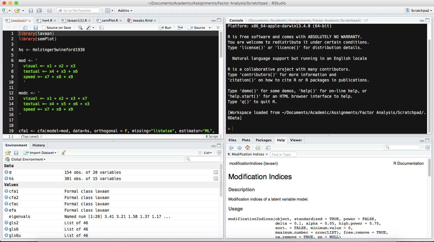
There are several customizations with my own setup compared to the default, but the basics are all there. In the 4 quadrants, going from left to right, top to bottom, you have:
- The file viewer. Here you can write your code in a script file for safekeeping and reuse or look at your data in spreadsheet format. In this screenshot, you can see my working script file. When you want to look at more than one file at a time, you can view them in a separate window.
- The console. This replaces using the terminal and is where you enter code and see the output. You can either type out your code here or highlight code in the file viewer and use a keyboard shortcut to have it automatically entered.
- The environment viewer. This just shows you a list of all the objects that are currently in R’s environment. There’s some jargon here, but let’s avoid the details for now. In the screenshot, I have two datasets visible. One is named
dand the otherhs. If I were to click on them, they would appear in spreadsheet format in the top left quadrant. - The bottom right quadrant is many things at once. There are several tabs, as you can see. The one I have open in the above screenshot is the Help tab, which allows me to look at R documentation without leaving the current window. At first, you will struggle to make use of this, but over time it becomes more and more useful. You can also use this quadrant as a file explorer and it is the place where any graphics you produce will appear.
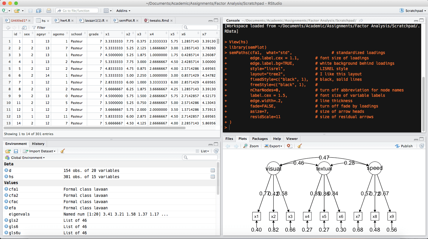
This is somewhat similar to the various views available in SPSS, but all in one window (which I find easier to keep track of). Below is another screen capture with a couple of the quadrants showing alternative versions of themselves (the data view on the top left and the plot view on the bottom right).
Step 2: Everything’s an object
Learning R as a coding language is less about remembering the specific syntax and more about grasping the underlying logic. Over time you will naturally start to commit the syntax you need to memory, but you’ll constantly struggle if you don’t know why it works the way it does.
I’ll gloss over and likely butcher the specific, computer science-y meaning of the terms, but R as a programming language can be object-oriented or functional. But in everyday usage for statistical purposes, it is predominantly object-oriented. This means in R you are constantly dealing with “objects.” This is just a catch-all for any kind of data.
Here’s a first code snippet:
num <- 5
What I’ve just done there is created an object called num which consists of the number 5. To assign a value to an object, just use the left pointing arrow (<-) followed by the value. This is the less-than sign and the hyphen on your keyboard. You can also use the regular equal sign (=) for the same purpose, but this is generally not recommended since there are a few situations in which this doesn’t work right.
If I want to use this value later for something else, I can refer to num instead of 5. You cannot use an object before it has been defined in some way. That is, if you just put num into the R console before assigning it a value, you will receive an error message. Once you have defined it, though, you can refer to it as much as you want.
num - 1
[1] 4
What comes in the second, lighter box is the output R would give in this situation, which is 4, the end result of 5 minus 1. For now, ignore the [1] but be aware it will be there on much of the output (it just means that 4 is the first result of num - 1, but of course there is only one result so it isn’t so helpful in this situation).
Something that is important to understand about this situation is that you have not changed num by subtracting 1, you have just asked R to tell you what would happen if you subtracted 1 from num. Here is some more code and output to illustrate:
num
[1] 5
num - 1
[1] 4
num
[1] 5
num <- num - 1

num
[1] 4
Okay, what did I do there at the end? I told R to change num to the value of num - 1, meaning the new value of num is 4. What this illustrates is that the object only changes if you specifically save the change to that object. Sometimes you’re just interested in what the result of something is (what is 5-1?) while other times you want to save that result for later.
Objects can store more than just numbers
As you might imagine, we wouldn’t need to bother with all of this if we just needed some way to keep track of numbers. Objects can store all kinds of data.
text <- "Some words"
Here I have created an object named text that stores a string of characters. This is a different type of object and I can’t do mathematical operations with it; text + 1 will cause an error. By putting things in quotation marks, I tell R that we’re dealing with a string (a set of characters in a particular order) rather than numbers. So even if I redefine text like this
text <- "5"
I can’t perform an operation like text + 1 since I have told R that text shouldn’t be treated like a number.
From here, it can get considerably more complex. I won’t show code examples for the moment, but your dataset is also going to be represented as an object. In R, your dataset is usually represented as what we call a “data frame,” which refers to the format in which your observations are in rows and the measured variables are in columns, just how they appear in SPSS or Excel. You will also save the results of your analyses in objects.
Some rules on naming
Before going too much further, there is something I should mention about R syntax. First of all, it is case sensitive. That means num and Num are two different objects. It is generally considered best practice to always name your objects with the first letter being lowercase, some of the reasons for which I won’t go into here. One of the reasons is obvious, though, in that it is harder to type out things with capital letters than it is with all lowercase.
For longer object names, some prefer to use “camel case” with the first segment lowercase, but with each other segment capitalized. For example, myTextObject is more readable than mytextobject.
You can use numbers, periods, and underscores in variable names, but only after the first letter. The first character must be a letter, but after that numbers are fine. Sometimes you may have an initial object called data or some such, but you tweak it and save the tweaked version as data2 or data_alt or data.alt. There is no minimum number of characters for an object name, so it is fine to call an object a or b, just remember that you’ll have to be able to remember what’s in there and sometimes a single letter isn’t expressive enough to remind you.
Vectors
If you’re like me before I started using R, the word “vector” is something I felt like I knew the meaning of but couldn’t quite wrap my head around what it would mean for an object in R to be a vector. Because R likes to think of data in terms of matrices, vectors are a common way data are represented. To put it in terms of matrices, a vector is a matrix that has 1 for one of its dimensions.
For instance, a 2x2 matrix is like this:
1 2
1 2
We can say that the 2x2 matrix consists of two 2x1 column vectors, [1,1] and [2,2]. Generally speaking, an easy way to think of vectors is as ordered lists of values. Keep in mind, however, that there is a specific data type known as a list, so use the word “vector” to refer to vectors.
Step 3: Know your functions
Most of the magic in R happens courtesy of functions. Functions perform a specific task on an object or set of objects. You use functions by writing out their name, a set of parentheses, and some arguments separated by commas inside the parentheses. What those arguments are depends on the function and how many instructions it needs.
Let’s start with the c() function, which is very useful for data manipulation. The “c” stands for “combine,” which is exactly what it does. Most of the time you want to save the result of the c() function to an object, which will be a vector. Here’s an example:
numVector <- c(1, 2, 3, 4, 5)
Now I have an object called numVector that is a vector of the numbers 1, 2, 3, 4, and 5. If I didn’t save it to an object, all R would do is print an output that says 1 2 3 4 5. Usually we want to do something with the result of our function, though, so we save it to an object.
For c(), the arguments can be any kinds of data and as many or as few of them as you desire.
Let’s look at another basic function, sum(). This, as you might have guessed, adds up data and reports the total. We can just provide it with values, like so:
sum(1,2)
[1] 3
We see that the output is 3, which is the same as doing this:
1 + 2
[1] 3
So you haven’t saved much time by using the sum() function in this case. But if you provide sum() with a numeric vector, it will add all the elements within it.
sum(numVector)
[1] 15
The alternatives to doing this are either
sum(1, 2, 3, 4, 5)
or
1 + 2 + 3 + 4 + 5
Those are perfectly fine, but if you plan on using that group of numbers for anything else then saving them as an object and inputting them into the function will save you a lot of time and help to prevent mistakes from typos.
Packages
R is different from SPSS in that only a subset of its capabilities are present by default. What some call “base” R is very capable, but if you are doing serious work you will eventually need more. The beauty of R is that third parties write and contribute functions that anyone can download and use. These functions are distributed in what are called “packages.”
Packages are just a set of functions written by a third party that you can download from CRAN, R’s central repository for packages. So if I wanted to install the psych package, which contains many functions useful for those doing social science research, I’d type this:
install.packages("psych")
And then R takes care of the rest. Now if I want to use one of those functions, I need load the package first. This tells R that if I type the name of a function that R hasn’t heard of, to look in this package to see if the package has that function. Suppose I want to use the psych package’s function called describe(), which prints the mean, standard deviation, and some other descriptive statistics all at once—with base R, you’d have to use separate functions for each of these pieces of information (mean(), sd(), and so on).
library(psych)
describe(numVector)
   vars n mean   sd median trimmed  mad min max range skew kurtosis   se
X1    1 5    3 1.58      3       3 1.48   1   5     4    0    -1.91 0.71
So now I have a bunch of descriptive statistics thanks to the describe() function of the psych package. It’s worth noting that once you have loaded the package, you don’t need to load it again until you have started a new R session (that is, you have closed R and opened it again).
In this example, the only argument I have provided to describe() is a numeric vector (numVector). However, there are other arguments I could provide. For instance, I might not want the calculation of skew and kurtosis. I can add an argument to eliminate that part of the output.
describe(numVector, skew=FALSE)
   vars n mean   sd min max range   se
X1    1 5    3 1.58   1   5     4 0.71
Now how would I know I could put this argument and get that result? Every function is documented. If I enter ?describe, I am shown the official documentation for that function, which includes a list of all the potential arguments I can provide along with brief explanations of what they do. The way this works is that the person who writes the function will specify the default for each argument and if you don’t enter anything else, the default will go in. So my first call to the describe() function didn’t mention the “skew” argument, so it assumed I wanted that information since that is the default. However, there is no default value for the data vector that I want descriptive statistics for, so I have to provide that or there will be an error.
It will take some practice to get used to reading documentation, so at first you will often need to rely on code examples you find on the internet or just experimenting to see what happens when you do certain things. Functions in base R also have documentation.
Step 4: Dealing with real datasets
My intended audience here is people who want to use R for social scientific data analysis, meaning you are probably already getting sick of my contrived examples with dummy data. Let’s talk about dealing with typical cases by variables datasets that experiments and surveys in the social sciences typically produce.
As luck would have it, R includes some pre-loaded example datasets that we can use for illustrative purposes. For now, we’ll use the dataset called attitude, which is already loaded into your R environment. A good practice, though, is to save it in a new data frame object.
att.data <- attitude
This dataset is 30 observations of 7 psychological variables. Type ?attitude to read the full documentation. If you just want to see how many observations and how many variables, use the dim() function. This means “dimensions.”
dim(att.data)
[1] 30 7
This means there are 30 rows and 7 columns in att.data.
What are these columns called, though? There are two ways to get acquainted. In RStudio, you can click on att.data in the environment list or enter the command View(att.data) in the console to see it spreadsheet-style in RStudio. Alternatively, you can uses the names() function to have the console print a list of the variable names for this data frame.
names(att.data)
[1] "rating"     "complaints" "privileges" "learning"   "raises"
[6] "critical"   "advance"
This can be handy for more than data frames too, but we’ll set that aside for the moment. R has printed out a list of all the names in their order. Note the numbers surrounded by brackets. This refers to the index of the value that follows it. So "rating" comes after [1], meaning "rating" is the first variable name for this data frame. "critical" comes after [6], meaning "critical" is the sixth variable name. As the lists get longer, this can be very helpful.
Referring to variables in a data frame
R has a particular way of accessing variables in a data frame object. From what I’ve told you thus far it isn’t obvious what you would do to perform an operation on just the complaints variable in the att.data data frame. There are two main ways to do this, but I’ll focus first on the most common and convenient way.
If I want to find the mean of complaints, I need to use the mean() function and give that function an argument that refers to complaints. To do that last part, we use the $ symbol. You start with the name of the data frame, then the dollar sign, then the variable name. Take a look:
mean(att.data$complaints)
[1] 66.6
By providing mean() with att.data$complaints as an argument, it knew to look in the att.data data frame for a variable named complaints. This is quite different than SPSS because in SPSS, there is only one dataset so it would be redundant to be constantly referring to it in your code or in the point-and-click interface. We’ll get to why R’s way of doing things can be useful in a bit. What is important, though, is that you can have an object called complaints that has nothing to do with the att.data data frame. You’re only referring to that variable when you write att.data$complaints. This can be especially helpful when you have a variable that shares a name with another R object or function. Imagine one of your variables was called mean or sum, for instance.
Using matrix indexing
An alternate way to single out a variable or an observation is by using matrix indexing. A data frame is basically a special type of matrix, so R understands what you mean when you tell it you want a certain row and/or column. Indexing refers to the act of accessing particular values by their numerical position in terms of rows and columns.
To do this, you use a format like this: dataframe[row,column]. So if I want the first variable (“rating”) for the first observation, I would enter:
att.data[1,1]
[1] 43
Okay, but we rarely want something so specific. To do the near-equivalent of att.data$rating, we can do this:
att.data[1]
   rating
1      43
2      63
3      71
4      61
5      81
I’ve cut off the output, but it goes on for 30 rows. When you enter just one digit in brackets after the dataframe, R generally assumes you want it to return the dataframe with only the 1st column.
What if I want all the variables, but just the first observation?
att.data[1,]
  rating complaints privileges learning raises critical advance
1     43         51         30       39     61       92      45
By adding a comma after the row index but then not adding a column index, R assumes that means I want everything for the specified row. The inverse applies as well; I can put just a comma and then the column index and get a list of the observations for a single column.
att.data[,1]
[1] 43 63 71 61 81 43 58 71 72 67 64 67 69 68 77 81 74 65 65 50 50 64 53 40 63
[26] 66 78 48 85 82
This is numerically equivalent to att.data[1] but it is returned as a numeric vector without any labels.
Additionally, you can specify a range of values for both rows and columns. Suppose I want just the 6th through 10th observations:
att.data[6:10,]
   rating complaints privileges learning raises critical advance
6      43         55         49       44     54       49      34
7      58         67         42       56     66       68      35
8      71         75         50       55     70       66      41
9      72         82         72       67     71       83      31
10     67         61         45       47     62       80      41
The colon operator means I want everything between 6 and 10. I won’t go into this level of detail in this post, but this indexing logic can be essential for efficiently subsetting data. You can specify, for instance, that you want to include only observations which have a certain level of att.data$complaints or some similar constraint and analyze those data separately.
Reading in data
Many people worry that switching to R means their existing data files will need replacing or some sort of special export in their native software, like SPSS. R has packages that are designed to read in all sorts of data, though.
In RStudio, you can actually do this with a point-and-click interface. In the latest version at the time of writing, RStudio gained the ability to deal with a great deal of file types, including SPSS’s .sav filetype.
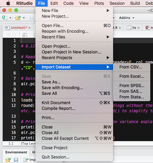
In the File menu, find “Import Dataset” and choose the relevant variant.
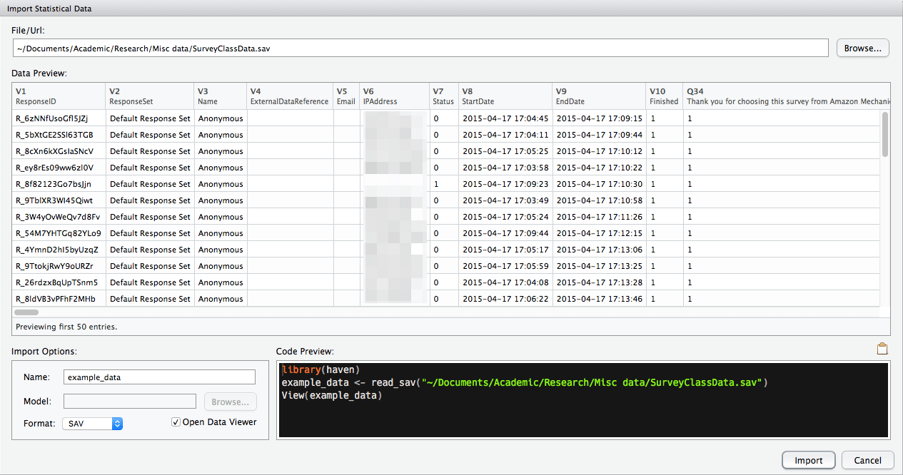
Using the window that appears next, find the file you’re looking for and it will show you a preview to help you make sure that it is reading the data correctly. You can choose from here what to name the data frame object. Take note of—and preferably save—the code preview so that you can reproduce the import in the future even if you don’t have RStudio handy or the options change.
From there, you’re pretty much ready to go!
Step 5: Your analysis lives in your script, not your output
Something I’ve never loved about SPSS is that in the way it is typically used, it is not the most conducive to reproducible work. Much of the time, we just save the output to a word document, especially if you are using the menus rather than the syntax editor. This can make it so tweaks to the analysis and even just reproducing analyses can be less than straightforward.
You can end up in the same traps with R, but it really pushes you towards more reproducible setups. There is no Word document to save and copy-pasting console output can go wrong in several ways. A better way of doing things is to keep everything you do in an R script file (.R file extension). And when I say everything, I mean everything from reading in the data, to naming variables, and of course every meaningful portion of the analysis.
When your analysis lives in a script file, you can just run the entire file at once to redo every last bit of it. R runs very quickly except when asked to deal with very large datasets (think larger than what SPSS allows) and so it generally takes just seconds to reproduce all the analyses that go into a typical social psychology article.
My analyses live in R Markdown files nowadays, but that’s beyond the scope of this article and is the same principle.
Additional resources for getting started
I don’t mean for this to be a comprehensive guide, but rather something to (comparatively) efficiently fill the gaps in many of the resources I used back when I had to learn R. Here are some other good places to go to get yourself going:
- The Personality Project’s documentation for getting started with R for psychological research is excellent and very detailed. I highly recommend it. These are the developers of the
psychpackage. - DataCamp has several free courses (like this one) that give you an interactive tutorial that doesn’t even require you to download R right away.
- Quick-R is filled with code examples organized by the specific tasks you might want to do, like linear regression, data cleaning, and so on.
- Roel Hogervost has a nice series on making the switch with many detailed examples. Here’s a link to part 1.
- RStudio has created several cheatsheets to act as a quick reference to frequently used syntax.
- R4Stats, where you can find books on switching over, blog posts, and an early version of the book for free.
- RSeek is a search engine designed to only return results germane to R, which can be trickier than it sounds with normal search engines.