A new package for panel data analysis in R
It has been a long time coming, but my R package
panelr is now on
CRAN. Since I started work on it
well over a year ago, it has become essential to my own workflow and I hope
it can be useful for others.
panel_data object class
One key contribution, that I hope can help other developers, is the creation of
a panel_data object class. It is a modified tibble, which is itself a
modified data.frame. panel_data frames are grouped by entity, so many
operations (e.g., mean(), cumsum()) performed by dplyr’s mutate()
are groupwise operations. The panel_data frame also works very hard to
stay in sequential order to ensure that lag and lead operations within
mutate() make sense.
panel_data frames are in “long” format, in which each row is a unique
combination of entity and time point. Let’s run through a quick example. First,
the package includes the example “raw’ dataset called WageData, which comes
from the Panel Study of Income Dynamics. This is what it looks like:
library(panelr)
data("WageData")
head(WageData)
  exp wks occ ind south smsa ms fem union ed blk   lwage t id
1   3  32   0   0     1    0  1   0     0  9   0 5.56068 1  1
2   4  43   0   0     1    0  1   0     0  9   0 5.72031 2  1
3   5  40   0   0     1    0  1   0     0  9   0 5.99645 3  1
4   6  39   0   0     1    0  1   0     0  9   0 5.99645 4  1
5   7  42   0   1     1    0  1   0     0  9   0 6.06146 5  1
6   8  35   0   1     1    0  1   0     0  9   0 6.17379 6  1
The key columns are id and t. They tell you which respondent and which
time point the row refers to, respectively. Let’s convert it into a panel_data
frame.
wages <- panel_data(WageData, id = id, wave = t)
wages
# Panel data:    4,165 x 14
# entities:      id [595]
# wave variable: t [1, 2, 3, ... (7 waves)]
   id        t   exp   wks   occ   ind south  smsa    ms   fem union    ed
   <fct> <dbl> <dbl> <dbl> <dbl> <dbl> <dbl> <dbl> <dbl> <dbl> <dbl> <dbl>
 1 1         1     3    32     0     0     1     0     1     0     0     9
 2 1         2     4    43     0     0     1     0     1     0     0     9
 3 1         3     5    40     0     0     1     0     1     0     0     9
 4 1         4     6    39     0     0     1     0     1     0     0     9
 5 1         5     7    42     0     1     1     0     1     0     0     9
 6 1         6     8    35     0     1     1     0     1     0     0     9
 7 1         7     9    32     0     1     1     0     1     0     0     9
 8 2         1    30    34     1     0     0     0     1     0     0    11
 9 2         2    31    27     1     0     0     0     1     0     0    11
10 2         3    32    33     1     1     0     0     1     0     1    11
# ... with 4,155 more rows, and 2 more variables: blk <dbl>, lwage <dbl>
panel_data() needs to know the ID and wave columns so that it can protect them
(and you) against accidentally being dropped, re-ordered, and so on. It also
allows other panel data functions in the package to know this information
without you having to respecify every time.
Note that the wages data are grouped by id and sorted by t within each
id. That means when you want to do things like calculate group means and
create lagged variables, everything works correctly. A warning, though: this is
only true within mutate() and transmute() from the dplyr package.
library(dplyr)
wages %>%
  mutate(
    wks_mean = mean(wks), # this is the person-level mean
    wks_lag = lag(wks), # this will have a value of NA when t = 1
    cumu_wages = cumsum(exp(lwage)) # cumulative summation works within person
  ) %>%
  select(wks, wks_mean, wks_lag, lwage, cumu_wages)
# Panel data:    4,165 x 7
# entities:      id [595]
# wave variable: t [1, 2, 3, ... (7 waves)]
   id        t   wks wks_mean wks_lag lwage cumu_wages
   <fct> <dbl> <dbl>    <dbl>   <dbl> <dbl>      <dbl>
 1 1         1    32     37.6      NA  5.56       260.
 2 1         2    43     37.6      32  5.72       565.
 3 1         3    40     37.6      43  6.00       967.
 4 1         4    39     37.6      40  6.00      1369.
 5 1         5    42     37.6      39  6.06      1798.
 6 1         6    35     37.6      42  6.17      2278.
 7 1         7    32     37.6      35  6.24      2793.
 8 2         1    34     31.6      NA  6.16       475.
 9 2         2    27     31.6      34  6.21       975.
10 2         3    33     31.6      27  6.26      1500.
# ... with 4,155 more rows
Notice also that when you use select, the id and t columns ride along
even though you didn’t explicitly ask for them. The idea here is that it
isn’t a panel_data frame without them. It works the same way using base R
subsetting:
wages["wks"]
# Panel data:    4,165 x 3
# entities:      id [595]
# wave variable: t [1, 2, 3, ... (7 waves)]
   id        t   wks
   <fct> <dbl> <dbl>
 1 1         1    32
 2 1         2    43
 3 1         3    40
 4 1         4    39
 5 1         5    42
 6 1         6    35
 7 1         7    32
 8 2         1    34
 9 2         2    27
10 2         3    33
# ... with 4,155 more rows
You can get just the one column using double brackets or the $ subsetting
method. But note that using base R sub-assignment, you don’t need to sweat those
extra columns:
wages["wage"] <- exp(wages[["lwage"]]) # note double brackets
Describing panel data
I’m also working on building out some descriptive functionality just for
panel data. panel_data objects have a summary() method, which works best
when you have the skimr package installed. By default, it will provide
descriptive statistics for each column in each wave. To shorten the output,
you can choose columns using dplyr::select() style syntax.
summary(wages, union, lwage)
Variable type: numeric
| skim_variable | t | missing | complete | n | mean | sd | p0 | p25 | p50 | p75 | p100 | hist |
|---|---|---|---|---|---|---|---|---|---|---|---|---|
| union | 1 | 0 | 595 | 595 | 0.36 | 0.48 | 0.00 | 0.00 | 0.00 | 1.00 | 1.00 | ▇▁▁▁▅ |
| union | 2 | 0 | 595 | 595 | 0.35 | 0.48 | 0.00 | 0.00 | 0.00 | 1.00 | 1.00 | ▇▁▁▁▅ |
| union | 3 | 0 | 595 | 595 | 0.37 | 0.48 | 0.00 | 0.00 | 0.00 | 1.00 | 1.00 | ▇▁▁▁▅ |
| union | 4 | 0 | 595 | 595 | 0.37 | 0.48 | 0.00 | 0.00 | 0.00 | 1.00 | 1.00 | ▇▁▁▁▅ |
| union | 5 | 0 | 595 | 595 | 0.37 | 0.48 | 0.00 | 0.00 | 0.00 | 1.00 | 1.00 | ▇▁▁▁▅ |
| union | 6 | 0 | 595 | 595 | 0.36 | 0.48 | 0.00 | 0.00 | 0.00 | 1.00 | 1.00 | ▇▁▁▁▅ |
| union | 7 | 0 | 595 | 595 | 0.37 | 0.48 | 0.00 | 0.00 | 0.00 | 1.00 | 1.00 | ▇▁▁▁▅ |
| lwage | 1 | 0 | 595 | 595 | 6.38 | 0.39 | 5.01 | 6.12 | 6.42 | 6.65 | 6.91 | ▁▂▃▇▇ |
| lwage | 2 | 0 | 595 | 595 | 6.47 | 0.36 | 5.01 | 6.24 | 6.53 | 6.75 | 6.91 | ▁▁▂▅▇ |
| lwage | 3 | 0 | 595 | 595 | 6.60 | 0.45 | 4.61 | 6.33 | 6.61 | 6.86 | 8.27 | ▁▂▇▃▁ |
| lwage | 4 | 0 | 595 | 595 | 6.70 | 0.44 | 5.08 | 6.44 | 6.72 | 6.96 | 8.52 | ▁▃▇▂▁ |
| lwage | 5 | 0 | 595 | 595 | 6.79 | 0.42 | 5.27 | 6.51 | 6.80 | 7.04 | 8.10 | ▁▂▇▅▁ |
| lwage | 6 | 0 | 595 | 595 | 6.86 | 0.42 | 5.66 | 6.60 | 6.91 | 7.11 | 8.16 | ▁▃▇▃▁ |
| lwage | 7 | 0 | 595 | 595 | 6.95 | 0.44 | 5.68 | 6.68 | 6.98 | 7.21 | 8.54 | ▁▅▇▂▁ |
You can stop getting per-wave statistics by setting by.wave = FALSE. For
panels with many fewer entities, you might also want per-entity statistics. You
can achieve this by setting by.wave = FALSE and by.id = TRUE.
You can also visualize trends in your data using line_plot().
line_plot(wages, lwage)
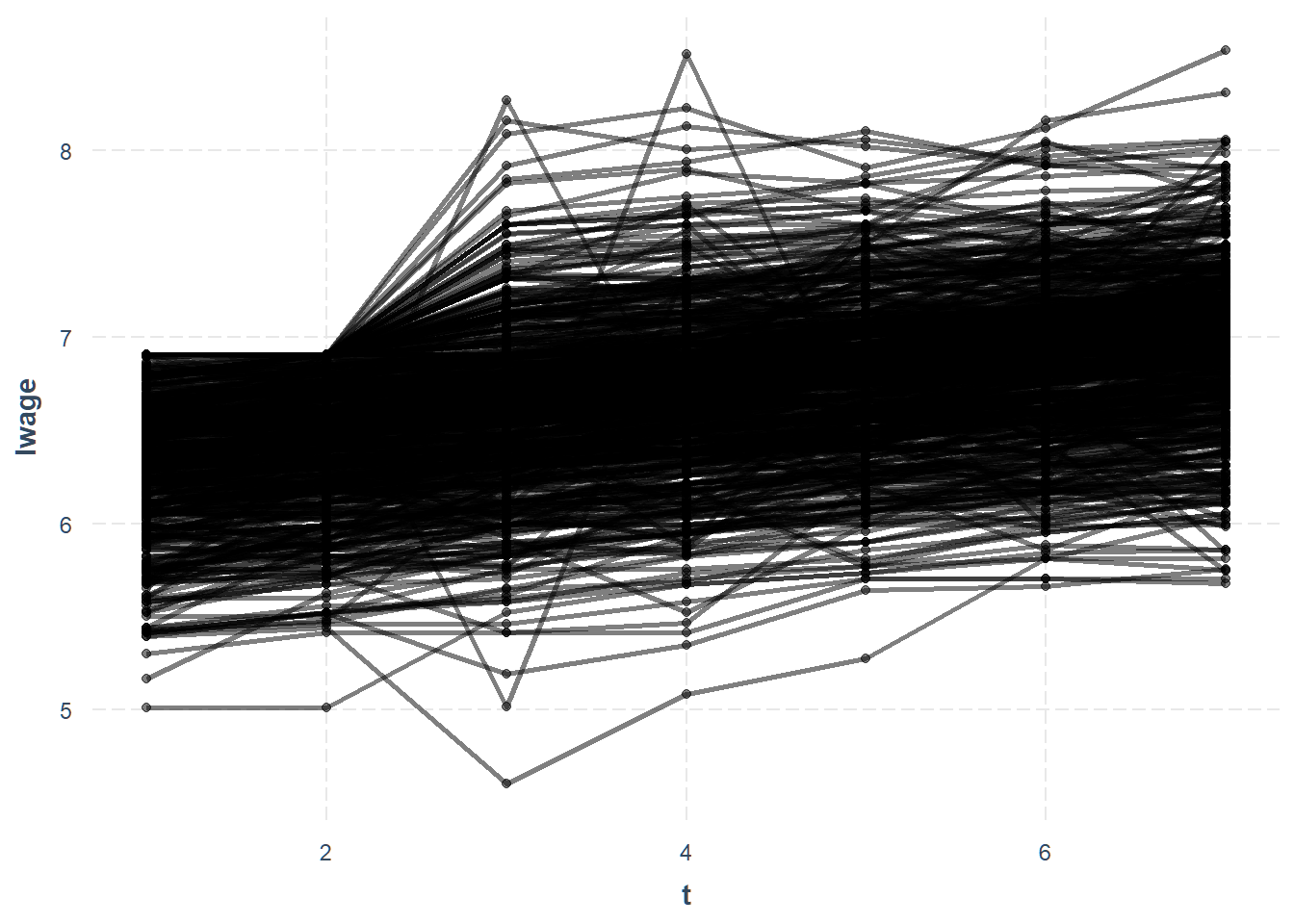
Each line is an individual id in the data.
Let’s see what the mean trend
looks like. While we’re at it, let’s make the individual lines a little more
transparent using the alpha argument.
line_plot(wages, lwage, add.mean = TRUE, alpha = 0.2)

The blue line is the mean trend and we can see that nearly everyone increases over time.
Sometimes it is useful to isolate specific entities from your data. I’ll use a different example to illustrate. These data come from the Penn World Table and contain data about countries, their exchange rates, purchasing power parity, and related data. It is provided by Stata and discussed in its manual.
library(haven)
penn <- read_dta("http://www.stata-press.com/data/r13/pennxrate.dta")
penn <- panel_data(penn, id = country, wave = year)
penn
# Panel data:    5,134 x 10
# entities:      country [151]
# wave variable: year [1970, 1971, 1972, ... (34 waves)]
   country  year xrate   ppp    id  capt realxrate lnrxrate  oecd    g7
   <fct>   <dbl> <dbl> <dbl> <dbl> <dbl>     <dbl>    <dbl> <dbl> <dbl>
 1 AFG      1970  45   10.8      1    34     1         0        0     0
 2 AFG      1971  45   11.2      1    34     0.250    -1.39     0     0
 3 AFG      1972  45    9.58     1    34     0.213    -1.55     0     0
 4 AFG      1973  45    8.94     1    34     0.199    -1.62     0     0
 5 AFG      1974  45    9.52     1    34     0.211    -1.55     0     0
 6 AFG      1975  45    9.12     1    34     0.203    -1.60     0     0
 7 AFG      1976  45    8.97     1    34     0.199    -1.61     0     0
 8 AFG      1977  45    9.33     1    34     0.207    -1.57     0     0
 9 AFG      1978  45    9.44     1    34     0.210    -1.56     0     0
10 AFG      1979  43.7  9.54     1    34     0.218    -1.52     0     0
# ... with 5,124 more rows
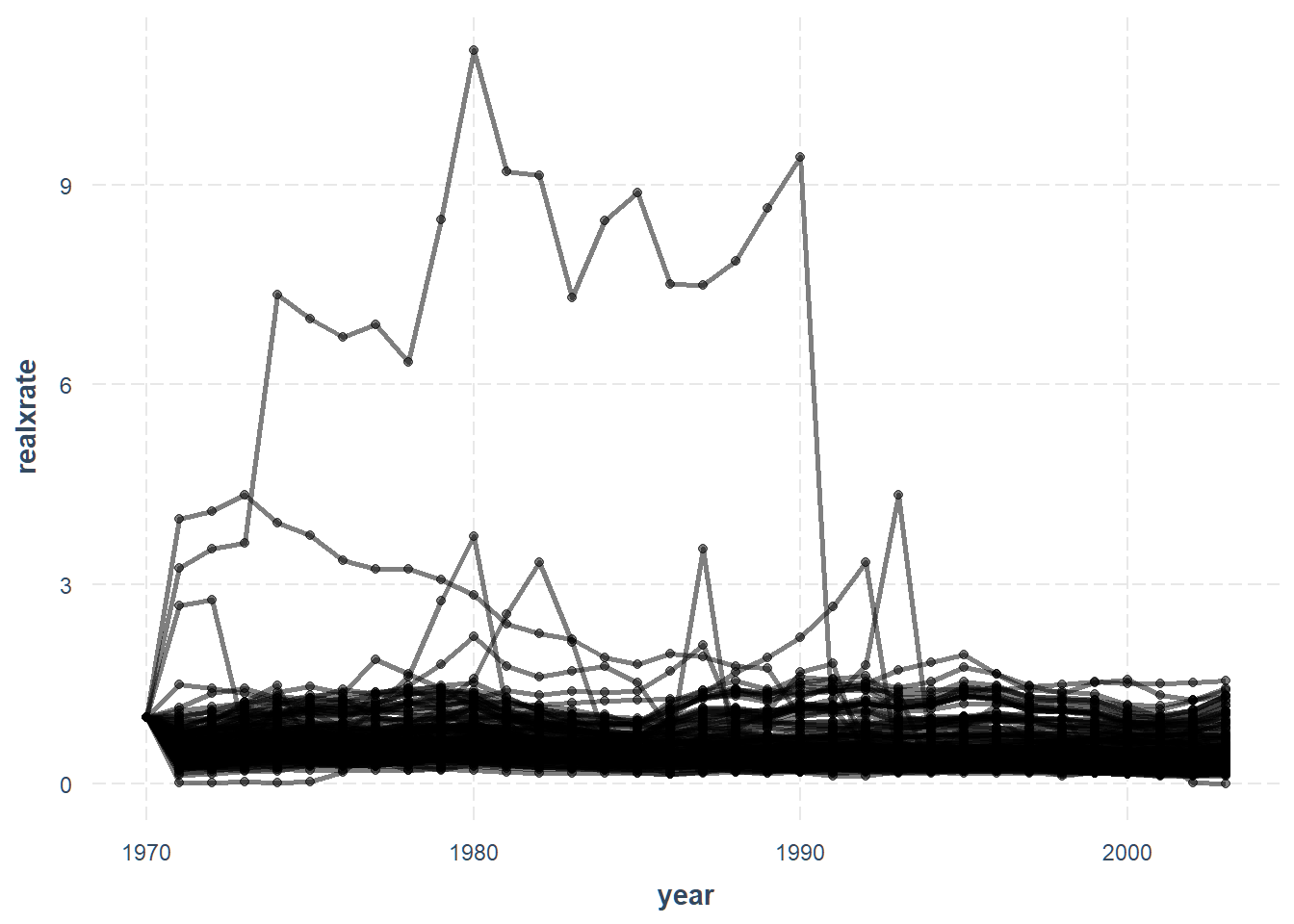
We’ll look at trends in the real exchange rate with the United States
(realxrate).
line_plot(penn, realxrate)
We can also look at each country separately by setting overlay = FALSE.
Since there are so many, we will want to look at just a subset. I’ll look at
members of the “G7” countries, minus the USA.
line_plot(penn, realxrate, overlay = FALSE,
          subset.ids = filter(penn, g7 == 1)$country, add.mean = TRUE)
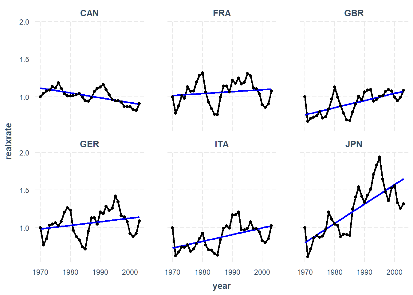
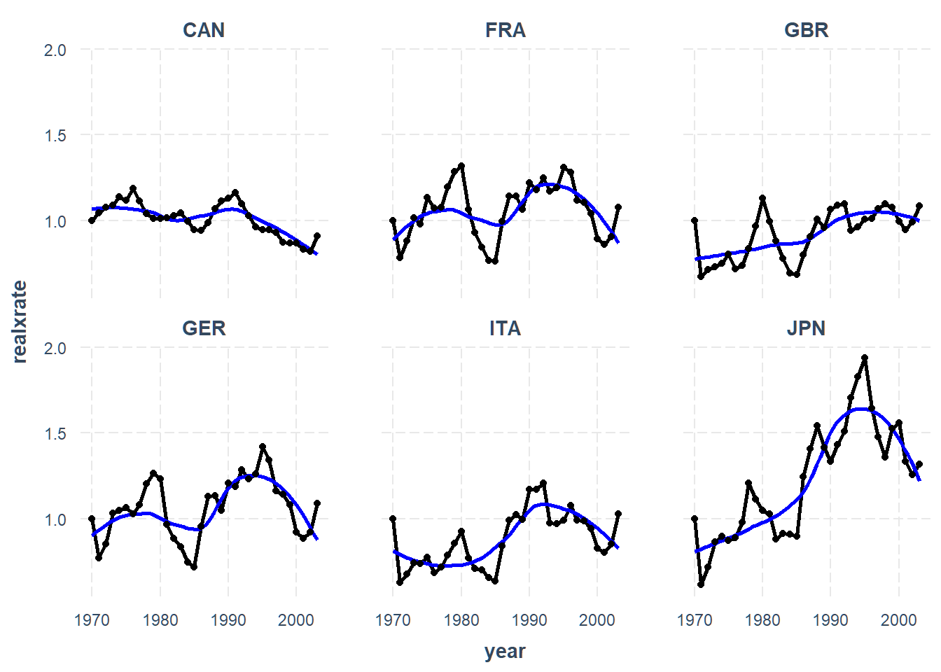
We can see some heterogeneity in the trends. You may also want to fit a
trend line that isn’t strictly linear, which is doable via the mean.function
argument.
line_plot(penn, realxrate, overlay = FALSE,
          subset.ids = filter(penn, g7 == 1)$country,
          add.mean = TRUE, mean.function = "loess")
Tools for reshaping data
Although you can get a much more detailed walk-through in the package’s
tutorial vignette,
I also want to mention some tools I created to help people
get their data into the long format demanded by panel_data() (and most
methods of analysis) as well as out of long format into a wide format in
which there is just 1 row per entity.
There are a number of tools that can do this, most notably base R’s reshape()
function. The problem with reshape() is that it can be a real pain to use,
especially if you have a lot of time-varying variables and/or they aren’t
labeled in a way congenial to what the function is looking for. The tidyr
package is also designed to help with problems like these, but I (and
apparently many
others)
struggle with the featured spread() and gather() functions, which in the
case of panel data have a tendency to make the data longer than you actually
want it unless you’re careful. They are great general tools, but my goal was
to make a specific tool to make life easier in this particular situation.
Going from long to wide format is fairly straightforward. Let’s take our
wages data. As a reminder, it looks like this:
wages
# Panel data:    4,165 x 15
# entities:      id [595]
# wave variable: t [1, 2, 3, ... (7 waves)]
   id        t   exp   wks   occ   ind south  smsa    ms   fem union    ed
   <fct> <dbl> <dbl> <dbl> <dbl> <dbl> <dbl> <dbl> <dbl> <dbl> <dbl> <dbl>
 1 1         1     3    32     0     0     1     0     1     0     0     9
 2 1         2     4    43     0     0     1     0     1     0     0     9
 3 1         3     5    40     0     0     1     0     1     0     0     9
 4 1         4     6    39     0     0     1     0     1     0     0     9
 5 1         5     7    42     0     1     1     0     1     0     0     9
 6 1         6     8    35     0     1     1     0     1     0     0     9
 7 1         7     9    32     0     1     1     0     1     0     0     9
 8 2         1    30    34     1     0     0     0     1     0     0    11
 9 2         2    31    27     1     0     0     0     1     0     0    11
10 2         3    32    33     1     1     0     0     1     0     1    11
# ... with 4,155 more rows, and 3 more variables: blk <dbl>, lwage <dbl>,
#   wage <dbl>
Let’s widen it, which will leave us with one row for each id.
widen_panel(wages)
# A tibble: 595 x 74
   id      fem    ed   blk exp_1 wks_1 occ_1 ind_1 south_1 smsa_1  ms_1
   <fct> <dbl> <dbl> <dbl> <dbl> <dbl> <dbl> <dbl>   <dbl>  <dbl> <dbl>
 1 1         0     9     0     3    32     0     0       1      0     1
 2 2         0    11     0    30    34     1     0       0      0     1
 3 3         0    12     0     6    50     1     1       0      0     1
 4 4         1    10     1    31    52     1     0       0      1     0
 5 5         0    16     0    10    50     1     0       0      0     1
 6 6         0    12     0    26    44     1     1       0      1     1
 7 7         0    12     0    15    46     1     0       0      0     1
 8 8         0    10     0    23    51     1     1       1      0     1
 9 9         0    16     0     3    50     0     0       1      1     1
10 10        0    16     0     3    49     0     0       1      1     1
# ... with 585 more rows, and 63 more variables: union_1 <dbl>,
#   lwage_1 <dbl>, wage_1 <dbl>, exp_2 <dbl>, wks_2 <dbl>, occ_2 <dbl>,
#   ind_2 <dbl>, south_2 <dbl>, smsa_2 <dbl>, ms_2 <dbl>, union_2 <dbl>,
#   lwage_2 <dbl>, wage_2 <dbl>, exp_3 <dbl>, wks_3 <dbl>, occ_3 <dbl>,
#   ind_3 <dbl>, south_3 <dbl>, smsa_3 <dbl>, ms_3 <dbl>, union_3 <dbl>,
#   lwage_3 <dbl>, wage_3 <dbl>, exp_4 <dbl>, wks_4 <dbl>, occ_4 <dbl>,
#   ind_4 <dbl>, south_4 <dbl>, smsa_4 <dbl>, ms_4 <dbl>, union_4 <dbl>,
#   lwage_4 <dbl>, wage_4 <dbl>, exp_5 <dbl>, wks_5 <dbl>, occ_5 <dbl>,
#   ind_5 <dbl>, south_5 <dbl>, smsa_5 <dbl>, ms_5 <dbl>, union_5 <dbl>,
#   lwage_5 <dbl>, wage_5 <dbl>, exp_6 <dbl>, wks_6 <dbl>, occ_6 <dbl>,
#   ind_6 <dbl>, south_6 <dbl>, smsa_6 <dbl>, ms_6 <dbl>, union_6 <dbl>,
#   lwage_6 <dbl>, wage_6 <dbl>, exp_7 <dbl>, wks_7 <dbl>, occ_7 <dbl>,
#   ind_7 <dbl>, south_7 <dbl>, smsa_7 <dbl>, ms_7 <dbl>, union_7 <dbl>,
#   lwage_7 <dbl>, wage_7 <dbl>
Notice that for variables that vary over time, there is now a column for each wave.
Going from wide to long is a bit more complicated because you need to automate
the process of knowing how many waves there are, which variables change over
time, and how the time-varying variables are labeled to reflect the time of
the measurement. We’ll use another example dataset from this package, called
teen_poverty, that starts in the wide format.
data("teen_poverty")
teen_poverty
# A tibble: 1,151 x 28
      id  pov1 mother1 spouse1 inschool1 hours1  pov2 mother2 spouse2
   <dbl> <dbl>   <dbl>   <dbl>     <dbl>  <dbl> <dbl>   <dbl>   <dbl>
 1    22     1       0       0         1     21     0       0       0
 2    75     0       0       0         1      8     0       0       0
 3    92     0       0       0         1     30     0       0       0
 4    96     0       0       0         0     19     1       1       0
 5   141     0       0       0         1      0     0       0       0
 6   161     0       0       0         1      0     0       0       0
 7   220     0       0       0         1      6     0       0       0
 8   229     0       0       0         1      0     1       0       0
 9   236     0       0       0         1      0     0       0       0
10   240     0       0       0         1     18     1       0       0
# ... with 1,141 more rows, and 19 more variables: inschool2 <dbl>,
#   hours2 <dbl>, pov3 <dbl>, mother3 <dbl>, spouse3 <dbl>,
#   inschool3 <dbl>, hours3 <dbl>, pov4 <dbl>, mother4 <dbl>,
#   spouse4 <dbl>, inschool4 <dbl>, hours4 <dbl>, age <dbl>, black <dbl>,
#   pov5 <dbl>, mother5 <dbl>, spouse5 <dbl>, inschool5 <dbl>,
#   hours5 <dbl>
We have some variables that don’t change over time (like whether the respondent
is black) and a number that do, like whether the respondent is married
(spouse).
long_panel() needs to know what the waves are called (1, 2, 3, …),
where the wave label is in the variable name (beginning or end), and whether
the label has prefixes or suffixes (e.g., “W1_variable” has a “W” prefix and
“_” suffix). In this case, we have no prefix/suffix, the label is at the end,
and the labels go from 1 to 5.
long_panel(teen_poverty, label_location = "end", periods = 1:5)
# Panel data:    5,755 x 9
# entities:      id [1151]
# wave variable: wave [1, 2, 3, ... (5 waves)]
   id     wave   age black   pov mother spouse inschool hours
   <fct> <dbl> <dbl> <dbl> <dbl>  <dbl>  <dbl>    <dbl> <dbl>
 1 22        1    16     0     1      0      0        1    21
 2 22        2    16     0     0      0      0        1    15
 3 22        3    16     0     0      0      0        1     3
 4 22        4    16     0     0      0      0        1     0
 5 22        5    16     0     0      0      0        1     0
 6 75        1    17     0     0      0      0        1     8
 7 75        2    17     0     0      0      0        1     0
 8 75        3    17     0     0      0      0        1     0
 9 75        4    17     0     0      0      0        1     4
10 75        5    17     0     1      0      0        1     0
# ... with 5,745 more rows
Perfect! As a note, long_panel() does fairly well in more complicated
situations, like when time-varying variables are only measured in some waves
and not others. See the
vignette for more details.
Regression models
The other main contribution of the panelr package is that it provides
a straightforward way to fit some panel data regression models. These are,
by and large, doable via other common packages. The reason for implementing
them in panelr is that they typically require some programming that would
be difficult for novice and maybe even intermediate R users and even for the
best of us, can be error-prone.
The first and most important of these is what is often called the “within-between” or sometimes “between-within” and “hybrid” model, which separates within-entity and between-entity variance. The within-entity portion is equivalent to what econometricians called the “fixed effects” model. People like these models because they are robust to confounding by individual differences. You don’t have to measure income, or personality, or whatever it may be and it is automatically controlled for because each person serves as their own control. Unlike fixed effects models, however, you can still include stable variables if you’re interested in their effects.
And because the models are estimated via multilevel models, you can take advantage of the specification flexibility afforded by them with random slopes and so on.
You can learn in more detail what these models are all about in the package’s introductory vignette.
These models are implemented via the wbm() function
(within-between model). Let’s run through an example with
the teen_poverty data. First we’ll transform it to long format like in
the earlier example, then we’ll predict hours worked (hours) using indicators
of whether the respondent’s marital status changed (spouse), they
became a mother (mother), or have enrolled in school (inschool).
teen <- long_panel(teen_poverty, label_location = "end", periods = 1:5)
model <- wbm(hours ~ spouse + mother + inschool, data = teen)
summary(model)
MODEL INFO:
Entities: 1151
Time periods: 1-5
Dependent variable: hours
Model type: Linear mixed effects
Specification: within-between

MODEL FIT:
AIC = 45755.31, BIC = 45815.23
Pseudo-R² (fixed effects) = 0.15
Pseudo-R² (total) = 0.35
Entity ICC = 0.23

WITHIN EFFECTS:
--------------------------------------------------------
                   Est.   S.E.   t val.      d.f.      p
-------------- -------- ------ -------- --------- ------
spouse            -1.22   0.83    -1.47   4601.00   0.14
mother            -6.52   0.74    -8.76   4601.00   0.00
inschool         -11.09   0.47   -23.65   4601.00   0.00
--------------------------------------------------------

BETWEEN EFFECTS:
---------------------------------------------------------------
                          Est.   S.E.   t val.      d.f.      p
--------------------- -------- ------ -------- --------- ------
(Intercept)              20.38   0.76    26.87   1147.00   0.00
imean(spouse)            -1.53   1.29    -1.18   1147.00   0.24
imean(mother)            -9.83   0.90   -10.95   1147.00   0.00
imean(inschool)         -15.23   0.94   -16.27   1147.00   0.00
---------------------------------------------------------------

p values calculated using Satterthwaite d.f.

RANDOM EFFECTS:
------------------------------------
  Group      Parameter    Std. Dev.
---------- ------------- -----------
    id      (Intercept)     6.504
 Residual                   11.74
------------------------------------
We have within- and between-subject effects here. The within effects can be
interpreted as the effects of changes in spouse, mother, and inschool
on hours worked. The between effects (which are the individual-level means,
hence imean()) reflect how the overall level of the variables correspond
with the overall level of hours worked, but don’t tell us much about change
in either one.
From the output, we can see the within and between effects are quite similar. Unsurprisingly, starting school corresponds with a substantial decrease in hours worked as does becoming a mother.
What if we want to know about the effect of race? wbm() uses a multi-part
formula to allow you to explicitly specify stable variables. You separate
the within- and between-entity variables with a bar (|). For example:
model <- wbm(hours ~ spouse + mother + inschool | black, data = teen)
summary(model)
MODEL INFO:
Entities: 1151
Time periods: 1-5
Dependent variable: hours
Model type: Linear mixed effects
Specification: within-between

MODEL FIT:
AIC = 45755.79, BIC = 45822.37
Pseudo-R² (fixed effects) = 0.15
Pseudo-R² (total) = 0.35
Entity ICC = 0.23

WITHIN EFFECTS:
--------------------------------------------------------
                   Est.   S.E.   t val.      d.f.      p
-------------- -------- ------ -------- --------- ------
spouse            -1.22   0.83    -1.47   4601.00   0.14
mother            -6.52   0.74    -8.76   4601.00   0.00
inschool         -11.09   0.47   -23.65   4601.00   0.00
--------------------------------------------------------

BETWEEN EFFECTS:
---------------------------------------------------------------
                          Est.   S.E.   t val.      d.f.      p
--------------------- -------- ------ -------- --------- ------
(Intercept)              20.60   0.79    26.07   1146.00   0.00
imean(spouse)            -1.67   1.30    -1.29   1146.00   0.20
imean(mother)            -9.65   0.92   -10.54   1146.00   0.00
imean(inschool)         -15.15   0.94   -16.13   1146.00   0.00
black                    -0.52   0.51    -1.01   1146.00   0.31
---------------------------------------------------------------

p values calculated using Satterthwaite d.f.

RANDOM EFFECTS:
------------------------------------
  Group      Parameter    Std. Dev.
---------- ------------- -----------
    id      (Intercept)     6.504
 Residual                   11.74
------------------------------------
There does not seem to be a difference in hours worked between black and non-black respondents, at least after accounting for these other factors.
You can use a third part of the formula as well, where you can specify
cross-level interactions (i.e., within by between interactions) as well as
use the lme4 syntax for random effects (by default, (1 | id) is included
without you putting it into the formula). Here’s we will see if the effect
of becoming a mother is different for black and non-black respondents.
model <- wbm(hours ~ spouse + mother + inschool | black | black * mother, data = teen)
summary(model)
MODEL INFO:
Entities: 1151
Time periods: 1-5
Dependent variable: hours
Model type: Linear mixed effects
Specification: within-between

MODEL FIT:
AIC = 45735.34, BIC = 45808.58
Pseudo-R² (fixed effects) = 0.15
Pseudo-R² (total) = 0.35
Entity ICC = 0.24

WITHIN EFFECTS:
--------------------------------------------------------
                   Est.   S.E.   t val.      d.f.      p
-------------- -------- ------ -------- --------- ------
spouse            -0.87   0.83    -1.05   4600.00   0.30
mother           -10.78   1.21    -8.92   4600.00   0.00
inschool         -11.01   0.47   -23.51   4600.00   0.00
--------------------------------------------------------

BETWEEN EFFECTS:
---------------------------------------------------------------
                          Est.   S.E.   t val.      d.f.      p
--------------------- -------- ------ -------- --------- ------
(Intercept)              20.60   0.79    26.07   1146.00   0.00
imean(spouse)            -1.67   1.30    -1.29   1146.00   0.20
imean(mother)            -9.65   0.92   -10.54   1146.00   0.00
imean(inschool)         -15.15   0.94   -16.13   1146.00   0.00
black                    -0.52   0.51    -1.01   1146.00   0.31
---------------------------------------------------------------

CROSS-LEVEL INTERACTIONS:
----------------------------------------------------------
                     Est.   S.E.   t val.      d.f.      p
------------------ ------ ------ -------- --------- ------
mother:black         6.34   1.42     4.47   4600.00   0.00
----------------------------------------------------------

p values calculated using Satterthwaite d.f.

RANDOM EFFECTS:
------------------------------------
  Group      Parameter    Std. Dev.
---------- ------------- -----------
    id      (Intercept)     6.512
 Residual                   11.72
------------------------------------
Indeed, there seems to be.
There are a number of other things available for regression modeling of panel data that I will not cover in detail here — see the introductory vignette for more info. These include detrending variables in the within-between model, estimating within-between models with generalized estimating equations (GEE), first differences models, and asymmetric effects models in which increases and decreases over time are expected to have different effects.